Julio Sotelo | Time Series Analysis Forecasting

Time Series Analysis Forecasting

Summary

The objective this time is to show a simple and straightforward time series analysis including regressor for the predicted variable. The data was collected from Yahoo finance and from Federal Reserve bank of St. Louis (http://research.stlouisfed.org/fred2/). I am using R and libraries included with it to the task. Full code is provided.

Can stock price be predicted? Does the unemployment rate, inflation and personal consumption affect grocery store stock price? After analysing the historical Walmart stock price, we find out that the close stock price is not predicted by our final model including personal consumption and inflation. Walmart’s industry has little impact over significant shocks in the economy as it is personal budget or increasing prices. American households will not stop buying groceries just because they have a lower budget or grocery prices are higher.

In conclusion, Walmart stock price can’t be predicted by unemployment rate, personal consumption and the sports goods stores numbers. We might need further data such as craft beer consumption or other related data to make further analysis.

Exploratory Analysis

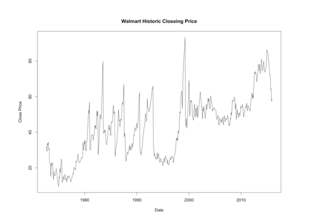
As part of the exploratory analysis of the closing price for Walmart stock listen in the NYSE, we see a that the time series has an upward trend. It does not follows a stationary process since the mean does not seem constant and the variance changes in time. For the most recent history, from 2000 to the end of 2015, the process has two major movements. The first one is from 2000 until the end of 2010 where it shows a stationary process. The second movement is and upward trend starting in 2011 that ends with a major shock at the end of 2015.
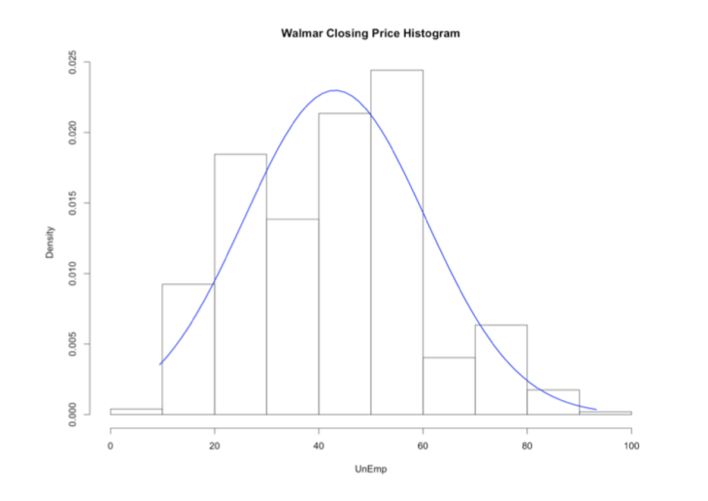
From the histogram we see a that the distribution is slightly skewed to the right, meaning that high prices for the stock are not commonly observed with a mean value of 43 dollars per share. The quantile plot show the thick left tail in comparison to the right tail in detail, see Appendix W1. Some basic statistics from the time series show confirms that the distribution is not symmetric; testing for normality with the Jarque-Bera we reject the hypothesis of a normal distribution.

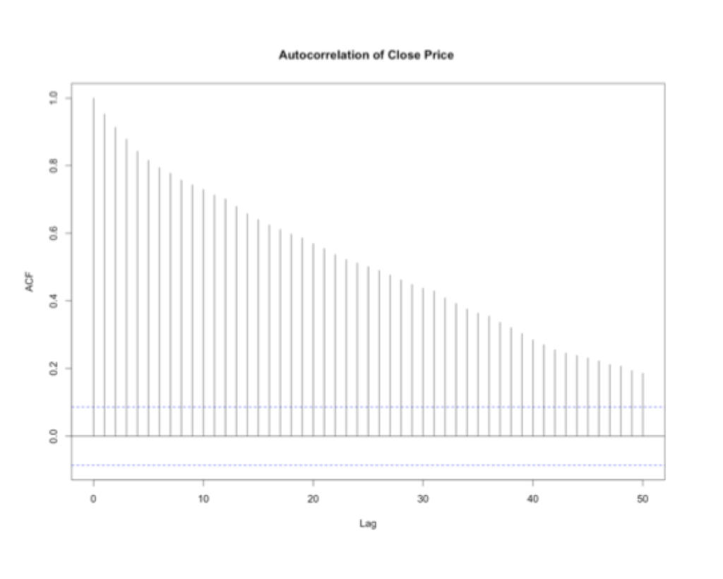
Looking at the autocorrelation that the time series its possible to see a strong serial correlation. The effect of one period extends for over 50 periods in time. That means that a high value is preceded by a high value and a low value is preceded by a low value even after 50 days. Performing a Ljung Box test for autocorrelation at lags 3, 5 and 7 there is significant evidence that the process is strongly auto correlated. This information is important since we may confirm that since the process is serially correlated we may try to find a model to predict the behavior and help us to tackle our first objective, predict Walmart’s stock price. The following step is to find a model that fits the overall process of the time series and test it for significance. To that end we use a tool in R that help to determine a proper model. It would test various models and select the best model based on the Bayesian Information Criterion BIC, see appendix W2 for results.

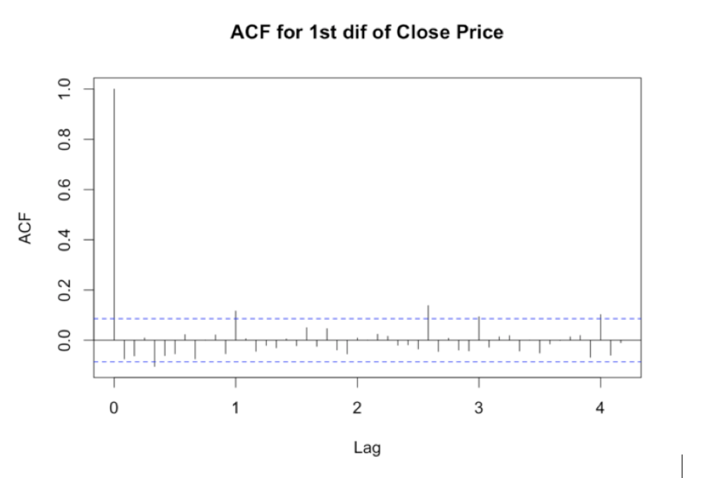
The suggested model has an autoregressive model (AR), a moving-average model (MA), a seasonal MA component with 1 year lag, and its suggesting to take the first difference of the data. From the autocorrelation function this final component was not so obvious, see appendix W3. However, it is likely that with the overall upward trend of the time series the difference would produce a positive effect trying to replicate the process.

Time series

Autocorrelation Function

Distribution

W3 – ACF

Data Preprocessing

The model should provide information and the answer to our goal which is to predict future prices for the sock. But we want to incorporate additional information such as personal consumption, unemployment rates and inflation in the United States. One problem with this is that the available information for stock prices, in general, are on daily basis for all business days; while the economic indicators that we have selected have monthly occurrences. To overcome that issue the price incorporated to the model is the first of the month, if that day was not a business day then the closest business day is selected.

Model Fitting

The model selection followed is with a backward approach. We start including all components and regressor to the model and if any of them has a bad fit it is removed or change from the previous model. For Walmart the initial model was set to with an AR(1,1,1) process with a seasonal component occurring every 12 months and a seasonal MA(1) and the three regressors were incorporated to the initial model. All the components but employment rates are significant and with consistent coefficients. In theory a final model have to include only significant, so following the backward approach we the next step is to remove unemployment rates who show no significance at our target level of 0.05. This second model turn out to be the final one. All components in the model are significant at the objective level, see appendix W4.

Fitted model

Residual Analysis

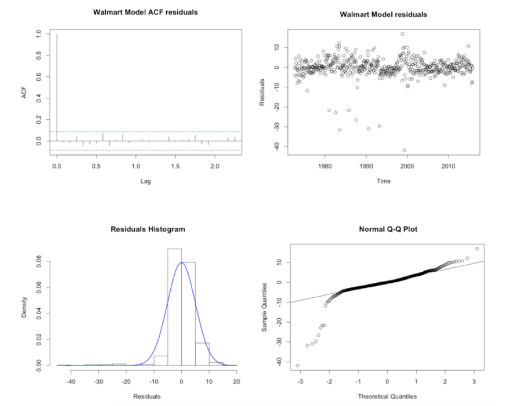
This final model show good residual behaviour. The Ljung-box test show no significant residuals different from zero. The distribution is normal with a long left tail as expected due to the distribution of the data, see appendix W5 for histogram, quantile plot, distribution, and autocorrelation function of residuals. The residuals are proven to be white noise. For further model validation backtest have been performed. To perform the backtest 80% of the data is used for training and 20% for testing. The analysis show that in average the predictions of the chosen model are 3.01% different than the actual value, measured with Mean Average Percentage Error MAPE.

Residual Analysis

Forecast

Since the model included values up to the end of 2015 Walmart stock prices for January and February can be predicted. The time series itself cover the values need by the SARIMA model. The values of the regresssor are the actual figures for January personal consumption and inflation. The results show that the prediction of January price was off by 3%, which is the expected value from the backtesting analysis. February show a difference of 13.6%.

Results and discussion

It is important to keep in mind that even when the model has good fit and MAPE conveys with the actual vs predicted 3% difference. The difference under the domain is poor one. A monthly difference in stock market of that magnitude is equivalent to a annual variation higher than 30%. These percentage is a good year performance of the S&P500 index.

R Code

library(rugarch);
library(tseries); library(fBasics); library(zoo); library(forecast); library(lmtest)
library(corrplot)
source('backtest.R')

 CPI
cpidata = read.csv('cpi.csv', header=T)

CPI_ts = ts(cpidata$CPI, start=c(1947,1),frequency = 12)
plot(CPI_ts, main ='Consumer Price Index', ylab = "CPI", xlab="Year")
# TS has a clear trend, non stationary proces

#crud_trend = stl(CPI_ts, s.window = "per")
#plot(crud_trend, main='Consumer Price Index CPI Trend')

# c) normal distribution test
par(mfrow = c(1,2), oma = c(0, 0, 0, 0))
hist(CPI_ts, xlab="CPI", prob=T, main="CPI Index Histogram")
xfit<-seq(min(CPI_ts),max(CPI_ts), length.out = 60)
yfit<-dnorm(xfit,mean=mean(CPI_ts),sd=sd(CPI_ts))
lines(xfit, yfit, col="blue", lwd=2)
qqnorm(CPI_ts, main= 'CPI Index Change Rate Normal Q-Q Plot')
qqline(CPI_ts, col = 'blue')
par(mfrow = c(1,1), oma = c(0, 0, 0, 0))
# Distribution seem somehow skewed… flat

# Kurtosis test
basicStats(CPI_ts)
k_stat = kurtosis(CPI_ts)/sqrt(24/length(CPI_ts))
print("Kurtosis test statistic")
k_stat
print("P-value = ")
2*(1-pnorm(abs(k_stat)))
# reject normality

#Skewness test, symmetry
skew_test = skewness(CPI_ts)/sqrt(6/length(CPI_ts))
skew_test # retuning the z-statistic value
2* (1-pnorm(abs(skew_test)))
# normality test
normalTest(CPI_ts,method=c("jb"))
# reject symmetry

# stationary?
acf(coredata(CPI_ts), plot=T, lag=150, main ='Autocorrelation of CPI Index' )
acf(coredata(CPI_ts), plot=F, lag=15, main ='Autocorrelation of CPI Index' )
# is not stationary, has strong serial correlation

#Partial acutocorrelation function to identify order
pacf(CPI_ts, main= 'CPI Index PACF')

# taking first difference
CPI_ts1d = diff(diff(CPI_ts,2))
plot(CPI_ts)
acf(CPI_ts1d,lag=150)
pacf(CPI_ts1d)

library(fUnitRoots)
adfTest(CPI_ts1d, lag=5 , type= 'ct')
adfTest(CPI_ts1d, lag=10 , type= 'ct')
adfTest(CPI_ts1d, lag=15 , type= 'ct')

#fitting the model automatically
CPIautomodel=auto.arima(CPI_ts1d, ic="bic", trace=T, stationary=T)
CPIautomodel

# With differencBest model: ARIMA(2,0,2)(0,0,1)[12] with zero mean

CPI_AutoModel=Arima(CPI_ts1d,order=c(2,0,2),seasonal=list(order=c(0,0,1),period=12), method="ML" , include.mean = T)
CPI_AutoModel
coeftest(CPI_AutoModel)

#residual analysis
par(mfrow = c(1,2), oma = c(0, 0, 0, 0))
acf(CPI_AutoModel$residuals, main = 'ARMA(1,2) residuals')
plot(CPI_AutoModel$residuals, type='p',main = 'ARMA(1,2) residuals')
par(mfrow = c(1,1), oma = c(0, 0, 0, 0))

# are redisuals white noise?
#lag = m, use something bellow 10 (5 or 7 normally) but be aware of the degrees of freedom
# they have to be larger than the number of parameters
Box.test(CPI_AutoModel$residuals, lag=7, type='Ljung', fitdf=5)
Box.test(CPI_AutoModel$residuals, lag=8, type='Ljung', fitdf=5)
Box.test(CPI_AutoModel$residuals, lag=10, type='Ljung', fitdf=5)

# Residuals histograms and normal quantile
par(mfrow = c(1,2), oma = c(0, 0, 0, 0))
hist(CPI_AutoModel$residuals, xlab="Residuals", prob=T, main="ARMA(1,2) Residuals Histogram")
xfit<-seq(min(CPI_AutoModel$residuals),max(CPI_AutoModel$residuals), length.out = 60)
yfit<-dnorm(xfit,mean=mean(CPI_AutoModel$residuals),sd=sd(CPI_AutoModel$residuals))
lines(xfit, yfit, col="blue", lwd=2)
qqnorm(CPI_AutoModel$residuals,main="ARMA(1,2) Normal Q-Q Plot")
qqline(CPI_AutoModel$residuals)
par(mfrow = c(1,1), oma = c(0, 0, 0, 0))

# COMPUTE ROOTS OF POLYNOMIAL & plot roots of polynomial in a unit-circle
polyroot(c(1,- CPI_AutoModel$coef[1:2]))
plot(CPI_AutoModel)

 Personal Consumption

PCdata = read.csv('PConsump.csv', header=T)
plot(PCdata)

PC_ts = ts(PCdata$PC, start=c(1959,1),frequency = 12)
plot(PC_ts, main ='Personal Consumption Services', ylab = "PC", xlab="Year")
# TS has a clear trend, non stationary proces

PCcrud_trend = stl(PC_ts, s.window = "per")
plot(PCcrud_trend, main='Personal Consumption Services Trend')

# c) normal distribution test
par(mfrow = c(1,2), oma = c(0, 0, 0, 0))
hist(PC_ts, xlab="PC", prob=T, main="PC Index Histogram")
xfit<-seq(min(PC_ts),max(PC_ts), length.out = 60)
yfit<-dnorm(xfit,mean=mean(PC_ts),sd=sd(PC_ts))
lines(xfit, yfit, col="blue", lwd=2)
qqnorm(PC_ts, main= 'PC Index Change Rate Normal Q-Q Plot')
qqline(PC_ts, col = 'blue')
par(mfrow = c(1,1), oma = c(0, 0, 0, 0))
# Distribution is skewed to the right…

# Kurtosis test
basicStats(PC_ts)
k_stat = kurtosis(PC_ts)/sqrt(24/length(PC_ts))
print("Kurtosis test statistic")
k_stat
print("P-value = ")
2*(1-pnorm(abs(k_stat)))
# has fat tails

#Skewness test, symmetry
skew_test = skewness(PC_ts)/sqrt(6/length(PC_ts))
skew_test # retuning the z-statistic value
2* (1-pnorm(abs(skew_test)))
# normality test
normalTest(PC_ts,method=c("jb"))
# reject symmetry

# stationary?
acf(coredata(PC_ts), plot=T, lag=150, main ='Autocorrelation of PC Index' )
acf(coredata(PC_ts), plot=F, lag=150, main ='Autocorrelation of PC Index' )
# is not stationary, has strong serial correlation

#Partial acutocorrelation function to identify order
pacf(PC_ts, main= 'PC Index PACF')

# taking first difference
PC_ts1d = diff(PC_ts,12)
plot(PC_ts)
acf(PC_ts1d,lag=150)
pacf(PC_ts1d)

adfTest(PC_ts1d, lag = 5, type = 'ct')
adfTest(PC_ts1d, lag = 9, type = 'ct')
adfTest(PC_ts1d, lag = 12, type = 'ct')

PC2 = diff(log(PC_ts))
plot(PC2)
plot(PC_ts)
plot(inflation)
plot(PC2)
acf(PC2)
pacf(PC2)
adfTest(PC2, lag = 5, type = 'c')
adfTest(PC2, lag = 9, type = 'c')
adfTest(PC2, lag = 12, type = 'c')

#fitting the model automatically fro the first difference
PCautomodel=auto.arima(PC_ts, ic="bic", trace=T)
PCautomodel

PC_AutoModel = Arima(PC2, order = c(1,1,1), method = "ML") # diff of the log (good residuals)
PC_AutoModel = Arima(PC_ts,order=c(1,2,1),seasonal=list(order=c(0,0,1),period=12), method="ML") # Raw TS (residual issues)
PC_AutoModel
coeftest(PC_AutoModel)

#residual analysis
par(mfrow = c(1,2), oma = c(0, 0, 0, 0))
acf(PC_AutoModel$residuals, main = 'ARMA(1,2) residuals')
plot(PC_AutoModel$residuals, type='p',main = 'ARMA(1,2) residuals')
par(mfrow = c(1,1), oma = c(0, 0, 0, 0))

# are redisuals white noise?
#lag = m, use something bellow 10 (5 or 7 normally) but be aware of the degrees of freedom
# they have to be larger than the number of parameters
Box.test(PC_AutoModel$residuals, lag=3, type='Ljung', fitdf=3)
Box.test(PC_AutoModel$residuals, lag=5, type='Ljung', fitdf=3)
Box.test(PC_AutoModel$residuals, lag=7, type='Ljung', fitdf=3)
Box.test(PC_AutoModel$residuals, lag=15, type='Ljung', fitdf=3)

 Unemployment
UnEmpdata = read.csv('Unemployment.csv', header=T)
plot(UnEmpdata)

UnEmp_ts = ts(UnEmpdata$UNRATE, start=c(1948,1),frequency = 12)
plot(UnEmp_ts, main ='Unemployment Rate', ylab = "Unemployment Rate", xlab="Year")
# TS has a clear trend, non stationary proces

Unemp_trend = stl(UnEmp_ts, s.window = "per")
plot(Unemp_trend, main='Unemployment Rate Trend')

# c) normal distribution test
par(mfrow = c(1,2), oma = c(0, 0, 0, 0))
hist(UnEmp_ts, xlab="UnEmp", prob=T, main="UnEmp Rate Histogram")
xfit<-seq(min(UnEmp_ts),max(UnEmp_ts), length.out = 60)
yfit<-dnorm(xfit,mean=mean(UnEmp_ts),sd=sd(UnEmp_ts))
lines(xfit, yfit, col="blue", lwd=2)
qqnorm(UnEmp_ts, main= 'UnEmp Rate Normal Q-Q Plot')
qqline(UnEmp_ts, col = 'blue')
par(mfrow = c(1,1), oma = c(0, 0, 0, 0))
# Distribution seem normal

# Kurtosis test
basicStats(UnEmp_ts)
k_stat = kurtosis(UnEmp_ts)/sqrt(24/length(UnEmp_ts))
print("Kurtosis test statistic")
k_stat
print("P-value = ")
2*(1-pnorm(abs(k_stat)))
# has thin tails

#Skewness test, symmetry
skew_test = skewness(UnEmp_ts)/sqrt(6/length(UnEmp_ts))
skew_test # retuning the z-statistic value
2* (1-pnorm(abs(skew_test)))
# normality test
normalTest(UnEmp_ts,method=c("jb"))
# reject symmetry

# stationary?
acf(coredata(UnEmp_ts), plot=T, lag=150, main ='Autocorrelation of UnEmp Index' )
acf(coredata(UnEmp_ts), plot=F, lag=150, main ='Autocorrelation of UnEmp Index' )
# is not stationary, has strong serial correlation

#Partial acutocorrelation function to identify order
pacf(UnEmp_ts, main= 'UnEmp Index PACF')

# taking first difference
UnEmp_ts1d = diff(UnEmp_ts,12)
plot(UnEmp_ts)
acf(UnEmp_ts1d,lag=20)
pacf(UnEmp_ts1d)

#fitting the model automatically
UnEmpautomodel=auto.arima(UnEmp_ts, ic="bic", trace=T)
UnEmpautomodel

UnEmp_AutoModel=Arima(UnEmp_ts1d,order=c(1,1,2),seasonal=list(order=c(0,0,2),period=12), method="ML")
UnEmp_AutoModel
coeftest(UnEmp_AutoModel)

#residual analysis
par(mfrow = c(1,2), oma = c(0, 0, 0, 0))
acf(UnEmp_AutoModel$residuals, main = 'ACF of residuals')
plot(UnEmp_AutoModel$residuals, type='p',main = 'ARMA(1,2) residuals')
par(mfrow = c(1,1), oma = c(0, 0, 0, 0))

# are redisuals white noise?
#lag = m, use something bellow 10 (5 or 7 normally) but be aware of the degrees of freedom
# they have to be larger than the number of parametersBox.test(UnEmp_AutoModel$residuals, lag=7, type='Ljung', fitdf=1)
Box.test(UnEmp_AutoModel$residuals, lag=7, type='Ljung', fitdf=5)
Box.test(UnEmp_AutoModel$residuals, lag=12, type='Ljung', fitdf=5)

# Residuals histograms and normal quantile
par(mfrow = c(1,2), oma = c(0, 0, 0, 0))
hist(UnEmp_AutoModel$residuals, xlab="Residuals", prob=T, main="ARMA(1,2) Residuals Histogram")
xfit<-seq(min(UnEmp_AutoModel$residuals),max(UnEmp_AutoModel$residuals), length.out = 60)
yfit<-dnorm(xfit,mean=mean(UnEmp_AutoModel$residuals),sd=sd(UnEmp_AutoModel$residuals))
lines(xfit, yfit, col="blue", lwd=2)
qqnorm(UnEmp_AutoModel$residuals,main="ARMA(1,2) Normal Q-Q Plot")
qqline(UnEmp_AutoModel$residuals)
par(mfrow = c(1,1), oma = c(0, 0, 0, 0))

# good fit fot unemployment

#=================================================================================
 Unemployment and inflation affect personal consumption and if so how big is the impact.
#=================================================================================

inflation = cpidata[146:828,2]
unemp = UnEmpdata$UNRATE[134:816]
consump = PC2
length(inflation)
length(unemp)
length(consump)

data = data.frame(inflation,unemp,consump)
cor(data)
plot(data)

modelb = Arima(consump, order=c(1,1,1), method="ML",
xreg=data.frame(data$inflation,data$unemp))
modelb = Arima(consump,order=c(1,1,2),seasonal=list(order=c(0,0,2),period=12), method="ML")
coeftest(modelb)

#residual analysis
par(mfrow = c(1,2), oma = c(0, 0, 0, 0))
acf(modelb$residuals, main = 'ARIMA(1,1,1) residuals')
plot(modelb$residuals, type='p',main = 'ARIMA(1,1,1) residuals')
par(mfrow = c(1,1), oma = c(4, 4, 10, 2))

# are redisuals white noise?
Box.test(modelb$residuals, lag=7, type='Ljung', fitdf=4)
Box.test(modelb$residuals, lag=8, type='Ljung', fitdf=4)
Box.test(modelb$residuals, lag=10, type='Ljung', fitdf=4)

# Residuals histograms and normal quantile
par(mfrow = c(1,2), oma = c(0, 0, 0, 0))
hist(modelb$residuals, xlab="Residuals", prob=T, main="ARIMA(1,1,1) Residuals Histogram")
xfit<-seq(min(modelb$residuals),max(modelb$residuals), length.out = 60)
yfit<-dnorm(xfit,mean=mean(modelb$residuals),sd=sd(modelb$residuals))
lines(xfit, yfit, col="blue", lwd=2)
qqnorm(modelb$residuals,main="ARIMA(1,1,1) Normal Q-Q Plot")
qqline(modelb$residuals)
par(mfrow = c(1,1), oma = c(0, 0, 0, 0))

#=================================================================================
#=================================================================================
 How does personal consumption impact Walmart’s stock price and how does unemployment rates affects Boston Beer Company??? stock price.
#=================================================================================
#=================================================================================

###################################################################################
 WALMART
###################################################################################

walmartdata= read.csv('Walmar&Consump.csv',header = T)
cor(walmartdata$Consump,walmartdata$Walmart)

walmartP = ts(walmartdata$Walmart,start=c(1972,9),frequency = 12)
plot(walmartP)
lines(walmartCP, col='blue')

##################################################################################
##################################################################################

walmartCP = ts(walmartdata$W_close,start=c(1972,9),frequency = 12)
plot(walmartCP, main = "Walmart Historic Closing Price" , ylab= 'Close Price' , xlab="Date")
Walmar2000 = walmartCP[329:520]
Walmar2000 = ts(Walmar2000,start=c(2000,1),frequency = 12)
walmartP = Walmar2000
plot(Walmar2000, main = 'Walmar Close Price 2000 – 2015')
walmart_rets = log(walmartP/lag(walmartP, -1))
plot(walmart_rets)

par(mfrow = c(1,2), oma = c(0, 0, 0, 0))
hist(walmartCP, xlab="Price", prob=T, main="Walmar Closing Price Histogram")
xfit<-seq(min(walmartCP),max(walmartCP), length.out = 60)
yfit<-dnorm(xfit,mean=mean(walmartCP),sd=sd(walmartCP))
lines(xfit, yfit, col="blue", lwd=2)
qqnorm(walmartCP, main= 'Walmar Closing Price Normal Q-Q Plot')
qqline(walmartCP, col = 'blue')
par(mfrow = c(1,1), oma = c(0, 0, 0, 0))

basicStats((walmartCP))
# Kurtosis test
k_stat = kurtosis(walmartCP)/sqrt(24/length(walmartCP))
print("Kurtosis test statistic")
k_stat
print("P-value = ")
2*(1-pnorm(abs(k_stat)))

#Skewness test, symmetry
skew_test = skewness(walmartCP)/sqrt(6/length(walmartCP))
skew_test # retuning the z-statistic value
2* (1-pnorm(abs(skew_test)))
normalTest(walmartCP,method=c("jb"))

Box.test(walmartCP,lag=3,type='Ljung')
Box.test(walmartCP,lag=5,type='Ljung')
Box.test(walmartCP,lag=7,type='Ljung')
# stationary?
acf(coredata(walmartCP), plot=T, lag=50, main ='Autocorrelation of Close Price ' )
# is not stationary, has strong serial correlation
#Partial acutocorrelation function to identify order
pacf(walmartCP, main= 'Walmart Close price PACF')
dif1= diff(walmartCP)
head(dif1)
acf(dif1, main= 'ACF for 1st dif of Close Price', lag = 50)

# plots PACF of squared returns to identify order of AR model
pacf(coredata(walmart_rets),lag=10)
#specify model using functions in rugarch package
#Fit ARMA(0,0)-GARCH(1,1) model
garch_spec = ugarchspec(variance.model=list(garchOrder=c(1,1),external.regressors = Wxreg),
mean.model=list(armaOrder=c(0,0)) )
#estimate model
garch11.fit=ugarchfit(spec=garch_spec, data=walmart_rets)
garch11.fit
#roling forecast
garch11.t.fit=ugarchfit(spec=garch_spec, data=walmart_rets, out.sample=100)
garch11.fcst=ugarchforecast(garch11.t.fit, n.ahead=5, n.roll=50)
garch11.fcst
plot(garch11.fcst)

#=================================================================================
# SARIMA Models
#=================================================================================
walmart_auto = auto.arima(walmart_rets, trace=T, ic="bic")
# Best model: ARIMA(1,1,1)(2,0,2)[12] for the retunrs.

walmartP_auto = auto.arima(walmartP, trace=T, ic="bic")
# Best model for walmart's Adj stock price: ARIMA(0,1,0) with drift
acf(coredata(walmartP), plot=T, lag=50 )

plot(walmartP)
# Is it relly unit root
adfTest(walmartP, lag=3 , type= 'ct')
adfTest(walmartP, lag=5 , type= 'ct')
adfTest(walmartP, lag=7 , type= 'ct')
# is stationary.

walmartCP_auto = auto.arima(walmartCP, trace=T, ic="bic")
# Best model for Walmart Close price: ARIMA(1,1,1)(0,0,1)[12]

pacf(walmartCP)
pacf(walmartdata$W_close)
#============
#============
# Regrssors for walmart Adj Price
constart = length(consump)-length(walmartP)+1
in_un_start = nrow(data)-length(walmartP)+1
Wxreg =data.frame(consump[constart:length(consump)], data$inflation[in_un_start:nrow(data)],
data$unemp[in_un_start:nrow(data)])
colnames(Wxreg)

# Non of the regressors are significant at level 5%, backward selection
Wxreg =data.frame(data$inflation[in_un_start:nrow(data)])
colnames(Wxreg)

#============ ARIMA(0,1,0) with drift
AjP_model = Arima(walmartP,order=c(0,1,0), include.drift = T,
method="ML",
xreg=Wxreg)
coeftest(AjP_model)
# Any good models were identify.

#============
#============
# Regrssors for walmart Close Price
# the initial model fitting consumption, inflation and unemployment do not need un emp
constart = length(consump)-length(walmartCP)+1
in_un_start = nrow(data)-length(walmartCP)+1
Wxreg = data.frame(consump[constart:length(consump)], data$inflation[in_un_start:nrow(data)],
data$unemp[in_un_start:nrow(data)])
colnames(Wxreg)

Wxreg_with_walmart = data.frame(walmartdata$W_close,consump[constart:length(consump)], data$inflation[in_un_start:nrow(data)],
data$unemp[in_un_start:nrow(data)])
colnames(Wxreg_with_walmart)

cor(Wxreg_with_walmart)
plot(Wxreg_with_walmart)

#=======================================
# second list of regregors
Wxreg1 = data.frame(consump[constart:length(consump)], data$inflation[in_un_start:nrow(data)])
colnames(Wxreg1) #============
CP_model = Arima(walmartCP,order=c(1,1,1),seasonal=list(order=c(0,0,1),period=12),
method="ML",
xreg=Wxreg1)
coeftest(CP_model)
summary(CP_model)
# residual analysis
par(mfrow = c(1,2), oma = c(0, 0, 0, 0));
acf(CP_model$residuals, main = 'Walmart Model ACF residuals');
plot(CP_model$residuals, type='p',main = 'Walmart Model residuals' , ylab='Residuals');
par(mfrow = c(1,1), oma = c(4, 4, 10, 2))
Box.test(CP_model$residuals, lag=7, type='Ljung', fitdf=5)
Box.test(CP_model$residuals, lag=8, type='Ljung', fitdf=5)
Box.test(CP_model$residuals, lag=10, type='Ljung', fitdf=5)
# Residuals histograms and normal quantile
par(mfrow = c(1,2), oma = c(0, 0, 0, 0))
hist(CP_model$residuals, xlab="Residuals", prob=T, main=" Residuals Histogram")
xfit<-seq(min(CP_model$residuals),max(CP_model$residuals), length.out = 60)
yfit<-dnorm(xfit,mean=mean(CP_model$residuals),sd=sd(CP_model$residuals))
lines(xfit, yfit, col="blue", lwd=2)
qqnorm(CP_model$residuals,main=" Normal Q-Q Plot")
qqline(CP_model$residuals)
par(mfrow = c(1,1), oma = c(0, 0, 0, 0))
## Backtest
Wlargo = length(walmartCP)
Wtraining_size= 0.8
orig = round(Wlargo*Wtraining_size,0)
backtest(CP_model, as.vector(walmartCP) ,orig = orig ,h=1, xre = Wxreg1)

aumption_Wxreg1 = data.frame()
f=forecast(CP_model,h= 1, xreg = Wxreg1, level=c(80,95))

Wxreg1_forcast = data.frame(c(0.002393067,-0.009231132), c(238.107,237.258))
colnames(Wxreg1_forcast) f = forecast.Arima(CP_model,xreg = Wxreg1_forcast)
f
plot(f, include = 150, main='Walmart Close Price Forecast')

WalmarJan = 61.46
WalmarFeb = 67.5

1- 59.57/WalmarJan
1- 58.3/WalmarFeb
s1 = ts(walmartdata$W_close, start=c(1972,9), freq=12)
# compute lower limit for 95% interval in original scale
lcl = ts(f$lower[,2], start=c(2016,1), freq=12)
# compute upper limit for 95% interval in original scale
ucl = ts(f$upper[,2], start=c(2016,1), freq=12)
# Forecast plot
plot(Walmar2000, main = 'Forecast', ylab = 'Price', xlab = 'Year', ylim=c(25, 100) )
lines(ts(c(f$fitted,f$mean), start=c(1972,9), freq=4), col="blue")
# it is strange that having a low MAPE during backtest, we actually see a very different forecast